Work in progress. I'm writing this alongside my audio ray tracer, so it grows with the project. Each part of the system is marked Working, In progress or Planned. Last updated 30 September 2026.
Introduction
Games simulate light in more and more detail, while sound propagation is still mostly authored by hand. The usual engine setup is a single line trace between listener and source, a lowpass filter when that line is blocked, and reverb volumes that someone places and tunes room by room. That works until the geometry changes. Open a door, blow a hole in a wall or add a room, and the audio doesn't know.
An audio ray tracer asks the level instead. It traces rays through the actual geometry, looks up what every surface is made of, and derives occlusion, transmission through walls and the reverb of the room from the result. This post walks through the systems and formulas that make that work, in the order the data flows through them. I'm building mine as an Unreal Engine plugin, but nothing here depends on the engine: any engine that can cast rays can do all of it.
If you know graphics path tracing, a lot will feel familiar. Cosine-weighted sampling, next-event estimation and Russian roulette all carry over (I compared the lighting versions in my post on MIS strategies). What changes is what a ray carries, and what you do with the result.
Sound is not light
Three differences shape everything that follows.
- Sound is slow. At 343 m/s, the echo from a wall 10 m away arrives almost 60 ms after you clap. Light transport can ignore time; sound can't, because when the energy arrives is the reverb. So the tracer keeps a histogram over time instead of a single sum.
- Wavelengths are huge. From 2.7 m at 125 Hz down to 8.6 cm at 4 kHz, sound waves are the size of the things they hit. A ray is only a good model when a surface is large compared to the wavelength, so rays work best at high frequencies and worst at low ones, where sound bends around obstacles (diffraction) and rooms ring at their resonant modes.
- Rays carry energy, not waves. A ray stores energy per frequency band and no phase. That makes the simulation cheap and stable, and it means interference effects such as room modes and comb filtering aren't simulated at all. This family of methods is called geometric acoustics.
The pipeline
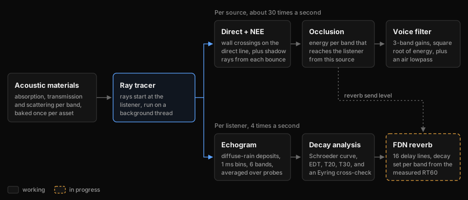
Everything starts with acoustic materials, baked once per asset. The ray tracer feeds two consumers. Per source, it estimates how much energy gets from that source to the listener in each frequency band, and that becomes a filter on the voice. Per listener, a separate room probe records when energy returns to the listener, which becomes an echogram, then a reverberation time, then the settings of a reverb.
The split is deliberate. How blocked a sound is depends on where its source is, so that has to be computed per source. How long a room rings doesn't depend on what's making the noise, so one probe per listener is enough. Tracing reverb-length paths for every source instead would cost roughly ten times as many line traces.
Frequency bands
Every quantity in the simulation is stored per frequency band. I use the six standard octave bands from 125 Hz to 4 kHz, because that's the resolution in which measured material data is published, and absorption varies a lot across them. That variation is most of what makes carpet sound different from concrete.
| Band | 125 Hz | 250 Hz | 500 Hz | 1 kHz | 2 kHz | 4 kHz |
|---|---|---|---|---|---|---|
| Wavelength | 2.74 m | 1.37 m | 69 cm | 34 cm | 17 cm | 8.6 cm |
Six is a simulation choice, not a DSP one. Another band costs the tracer one more float per ray, while the audio side pays per sample for every filter band, so the voice filter folds the six bands into three (more on that below).
Acoustic materials Working
When a ray hits a surface, the incident energy splits three ways. Some is absorbed (turned into heat), some is transmitted to the other side, and the rest is reflected. Per band $b$:
$$\alpha_b + \tau_b + \rho_b = 1 \quad\Longrightarrow\quad \rho_b = 1 - \alpha_b - \tau_b$$
A material asset stores three things:
- The absorption coefficient $\alpha_b$, taken from published tables measured in a reverberation room (ISO 354). Because it's measured rather than modelled, the asset treats it as ground truth.
- The transmission coefficient $\tau_b$, computed from physical properties: density, thickness and stiffness (next section).
- The scattering coefficient $s$: the fraction of reflected energy that leaves in a random, diffuse direction instead of the mirror direction (ISO 17497-1).
| Absorption $\alpha_b$ | 125 | 250 | 500 | 1k | 2k | 4k |
|---|---|---|---|---|---|---|
| Drywall on studs | 0.29 | 0.10 | 0.05 | 0.04 | 0.07 | 0.09 |
| Solid wood door | 0.14 | 0.10 | 0.06 | 0.08 | 0.10 | 0.10 |
| Carpet on concrete | 0.02 | 0.04 | 0.08 | 0.20 | 0.35 | 0.50 |
The table shows the materials in my test scene. Drywall absorbs mostly at 125 Hz, where the board and the cavity behind it resonate; carpet does the opposite and eats high frequencies. Two details matter more than they look.
First, the budget has to hold in every band. If $\alpha_b + \tau_b$ exceeds 1, the surface creates energy, so each asset checks this when it's baked, keeps the measured $\alpha_b$ and clamps the modelled $\tau_b$. Second, a measured absorption coefficient counts everything that isn't reflected back, and for a lightweight panel part of that is energy the panel passes to the other side, which is exactly what $\tau_b$ counts too. For heavy walls the overlap is negligible. For thin panels, $\rho_b = 1 - \alpha_b - \tau_b$ counts some of the same energy twice.
Scattering is the property I trust least. It depends on surface relief compared to the wavelength, not on what the surface is made of: a surface behaves as smooth when its bumps are smaller than about an eighth of a wavelength. The same oak can be a flat wall or a panelled door, and those scatter very differently. One scattering value per material, as I store it now, is a simplification.
Transmission through walls Working
Transmission is usually quoted as a transmission loss (TL) in decibels, while the simulation needs the energy ratio:
$$\tau = 10^{-\mathrm{TL}/10}$$
A 30 dB wall passes a thousandth of the energy. The interesting part is predicting TL from the physical properties of a wall.
The mass law
At low frequencies a wall behaves like a heavy, limp sheet. Sound pushes it back and forth, and the heavier it is, the less it moves. For sound arriving from all directions (the field-incidence mass law):
$$\mathrm{TL} \approx 20\log_{10}(m f) - 47\ \text{dB}$$
with $m$ the surface mass in kg/m² (density times thickness) and $f$ the frequency in Hz. Doubling the mass or the frequency buys 6 dB.
Coincidence
Real walls are stiff plates, and plates carry bending waves whose speed rises with frequency. At the critical frequency the bending waves travel exactly as fast as sound grazing along the surface, the two couple, and the wall suddenly becomes much easier to get through:
$$f_c = \frac{c^2}{2\pi}\sqrt{\frac{m}{B}}, \qquad B = \frac{E\,h^3}{12\,(1-\nu^2)}$$
Here $B$ is the bending stiffness of a thin plate with Young's modulus $E$ (not energy, for once), thickness $h$ and Poisson's ratio $\nu$. Around $f_c$ the transmission loss dips well below the mass law. Above it, the loss factor $\eta$ (the panel's internal damping, which depends heavily on how it's mounted) sets how quickly it recovers.
Sharp's model
Sharp's prediction method (1978) stitches these regions into one curve. With $\mathrm{TL}_A$ the value of the first line at $f_c/2$ and $\mathrm{TL}_B$ the value of the third line at $f_c$:
$$\mathrm{TL}(f) = \begin{cases} 20\log_{10}(m f) - 47 & f \lt f_c/2 \\[6pt] \mathrm{TL}_A + (\mathrm{TL}_B - \mathrm{TL}_A)\,\log_2\dfrac{2f}{f_c} & f_c/2 \le f \lt f_c \\[6pt] 20\log_{10}\dfrac{\pi m f}{\rho_0 c} + 10\log_{10}\dfrac{2\eta f}{\pi f_c} & f \ge f_c \end{cases}$$
Two details are easy to get wrong, and I got both wrong at first. The middle region is a straight line on a logarithmic frequency axis between its two neighbours, so the curve is continuous by construction. And above $f_c$ the curve is built on the normal-incidence mass law, $20\log_{10}(\pi m f / \rho_0 c) \approx 20\log_{10}(m f) - 42$ with $\rho_0 c \approx 415$ for air, not on the field-incidence one. That's a 5 dB difference.
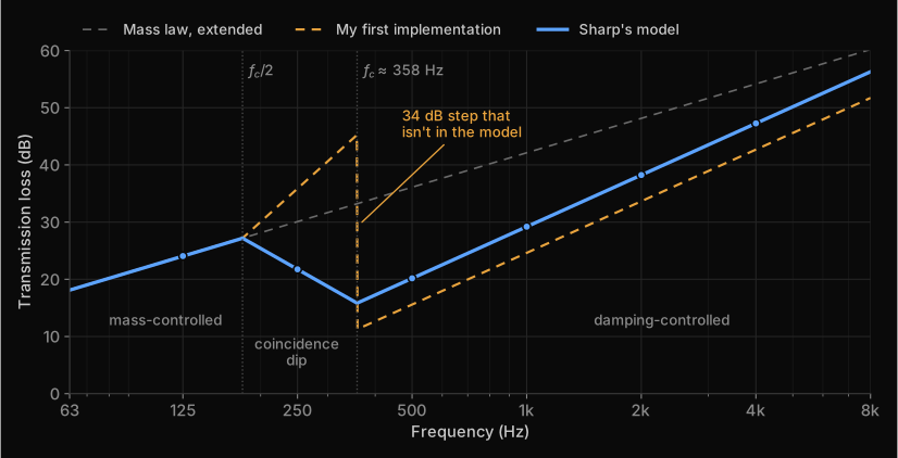
Pitfall. A piecewise model can be continuous on paper and discontinuous in code. Before trusting one, evaluate it just below and just above every breakpoint. My first version of this door jumped 34 dB at $f_c$ and put the 250 Hz band at 36 dB instead of 22 dB. A plot like the one above would have shown it in minutes.
Double walls
Most interior walls are two leaves with a cavity between them. The air in the cavity acts as a spring, which gives a mass-air-mass resonance:
$$f_0 = \frac{1}{2\pi}\sqrt{\frac{\rho_0 c^2\,(m_1 + m_2)}{d_{\text{cav}}\,m_1 m_2}}$$
Below $f_0$ the two leaves move together and the wall follows the mass law for its total mass. Above it they decouple, and transmission loss climbs at about 18 dB per octave until the cavity depth becomes comparable to the wavelength, where the slope drops to about 12 dB per octave. Studs and ties bridge the two leaves and cap the improvement.
Where the model stops working
Sharp's model assumes a large, thin, homogeneous panel with sound arriving from all directions at once. A ray tracer applies it per ray, at whatever angle the ray happens to hit, and to every material. That stretches it:
- Porous materials such as curtains, carpet or foliage transmit according to how easily air flows through them, not according to their mass.
- Small objects, around a wavelength or smaller, don't block sound at all; it bends around them.
- Gaps dominate everything. An opening of 1% of the area caps a wall at about 20 dB however heavy it is, and doors, windows and vents are full of gaps.
- Very light panels at low frequencies push the formula below 0 dB, which means nothing physically. Clamp TL at 0 dB: the panel passes everything.
There's a game-specific catch as well. A wall mesh is often a single-sided plane, so its thickness is a number someone typed into an asset. A more accurate model would mostly be more accurate about a guess, which is why I haven't moved to something heavier like the transfer matrix method.
Distance and air Working
Two things weaken sound over distance. The first is spreading. A point source spreads its power $W$ over a sphere, so intensity falls with the square of the distance, 6 dB per doubling:
$$I(d) = \frac{W}{4\pi d^2}$$
The second is air absorption, which turns sound into heat along the way. It's exponential in distance and strongly frequency dependent:
$$E(d) = E_0\,e^{-m_b d}, \qquad m_b = \frac{\ln 10}{10}\cdot\frac{a_b}{1000}$$
Standards publish the attenuation $a_b$ in dB per km. The second formula converts it to the energy coefficient $m_b$ per metre that the tracer uses. These are the values from ISO 9613-1 for 20 °C and 70% relative humidity:
| Band | 125 | 250 | 500 | 1k | 2k | 4k |
|---|---|---|---|---|---|---|
| $a_b$ (dB/km) | 0.3 | 1.1 | 2.8 | 5.0 | 9.0 | 22.9 |
| $m_b$ (1/m) | 0.00007 | 0.00025 | 0.00065 | 0.00115 | 0.00207 | 0.00527 |
Inside a building that's small for a single path, but it adds up in a reverb tail, where energy travels hundreds of metres. At 4 kHz it costs about 2.3 dB per 100 m. That's a large part of why real rooms decay faster at high frequencies, and why distant sounds are dull rather than just quiet. Humidity matters too: at 50% the 4 kHz value would be about 30 dB/km instead of 23.
Pitfall. Nepers come in an energy and an amplitude flavour. Converting dB/km with $\ln 10/20$ (amplitude) instead of $\ln 10/10$ (energy) halves the air absorption. And apply it exactly once per metre travelled: either along each segment or all at once when energy is deposited, never both.
In my plugin the room probe uses these coefficients directly. The direct path still uses a simpler distance-to-cutoff lowpass, which is much stronger than real air over the same distance; replacing it with these coefficients is on the list.
Energy in, amplitude out
Everything in the simulation is energy: absorption, transmission and air absorption are all energy ratios. Audio samples are pressure, and energy goes with pressure squared. So the moment a simulated number becomes a gain on a signal, it needs a square root:
$$g = \sqrt{\frac{E_{\text{out}}}{E_{\text{in}}}} \quad\Longleftrightarrow\quad 20\log_{10} g = 10\log_{10}\frac{E_{\text{out}}}{E_{\text{in}}}$$
Pitfall. Apply an energy ratio directly as an amplitude gain and every attenuation comes out twice as strong in decibels. My occlusion did exactly that for as long as the code existed. I now convert in one single place, where the simulation hands over to the audio, so it can't happen twice or not at all.
Tracing rays
Both consumers run the same bounce loop. They only differ in what they collect along the way.
Start at the listener
A game has one listener and many sources, so rays start at the listener. Energy transport is reciprocal: the path from A to B loses the same energy as the path from B to A. Tracing backwards gives the same answer and lets one set of rays serve every source.
Bouncing
At every hit the ray loses energy in each band and picks a new direction. With $\Delta d$ the length of the segment it just travelled:
$$E_b \leftarrow E_b\,\rho_b\,e^{-m_b\,\Delta d}$$
The scattering coefficient chooses the new direction. With probability $s$ the reflection is diffuse, otherwise it's a mirror reflection. Diffuse directions are sampled from a cosine-weighted hemisphere, Lambert's law, exactly like a diffuse surface in a path tracer:
$$\mathbf{d}_{\text{spec}} = \mathbf{d} - 2(\mathbf{d}\cdot\mathbf{n})\,\mathbf{n}, \qquad \mathbf{d}_{\text{diff}} = \big(\sqrt{u_1}\cos 2\pi u_2,\ \sqrt{u_1}\sin 2\pi u_2,\ \sqrt{1-u_1}\big)$$
Here $u_1, u_2$ are uniform random numbers and the diffuse direction is expressed in a frame around the normal $\mathbf{n}$. Picking one lobe at random instead of splitting the ray in two keeps the ray count constant, and on average it's the same thing.
Stopping
A ray could bounce forever, so it has to be stopped somehow. Cutting every ray off at a fixed depth is the obvious choice, and it's wrong: it silently deletes the end of the decay, which is exactly the part the reverb needs. Russian roulette stops rays without that bias. After a minimum depth, a ray survives with probability $q$, and a survivor's energy is divided by $q$ to make up for the rays that were killed:
$$E_b' = \begin{cases} E_b / q & \text{with probability } q \\ 0 & \text{with probability } 1 - q \end{cases} \qquad \mathbb{E}[E_b'] = q \cdot \frac{E_b}{q} = E_b$$
I start roulette at depth 10 with $q = \operatorname{clamp}(\max_b E_b,\ 0.05,\ 0.95)$. Rays with little energy left will probably die, and the ones that survive come back at full strength. The result is right on average; the price is noise, which the echogram averages away over time.
Pitfall. A maximum depth is still a truncation, even with roulette. The expected energy left after $n$ bounces is about $(1-\bar\alpha)^n$, so a cap of 64 bounces in a room with $\bar\alpha = 0.08$ cuts off everything below $10\log_{10}(0.92^{64}) \approx -23$ dB. That's inside the range you fit reverberation times on. With roulette in place the cap is only a safety net and can be generous, since very few rays ever get near it.
The whole loop
for each ray leaving the listener:
    E[b] = 1 for every band
    for depth = 0 .. maxDepth:
        hit = trace(origin, dir)              // nothing hit: energy left the level
        E[b] *= exp(-m[b] * hit.distance)     // air along this segment
        deposit(hit, E)                       // per-source NEE or room-probe rain
        E[b] *= rho[b]                        // absorption and transmission
        dir = rand() < s ? cosineSample(hit.normal) : reflect(dir, hit.normal)
        origin = hit.point
        if depth >= 10 and not roulette(E):   // survive with q, E /= q
            break
The next two sections are the two versions of deposit.
Occlusion per source Working
For every source, about 30 times a second, the tracer answers one question per band: how much of the source's energy reaches the listener, compared with an unobstructed path?
The direct path
First a straight line from listener to source. If it's clear, the direct transmission is 1 in every band. If it crosses walls, their transmission coefficients multiply, so their losses in decibels add:
$$D_b = \prod_{i\,\in\,\text{walls}} \tau_{i,b}$$
This ignores flanking, sound that goes around a wall through the building's structure, which in real buildings often decides what you actually hear from next door.
Paths around the obstacle
A sound behind a pillar isn't silent: it reaches you around the pillar, via reflections. To find those paths, rays leave the listener and bounce through the scene, and at every bounce the tracer casts a shadow ray straight at the source. This is next-event estimation, the same trick a path tracer uses for small lights. Instead of hoping a random bounce happens to hit a small target, you test the direct connection at every step.
For occlusion only the first connection of each ray counts. If ray $j$ first sees the source with energy $E_{j,b}$ after a total distance $d_j$, including the shadow ray, it contributes $C_{j,b} = E_{j,b}\,e^{-m_b d_j}$. A ray that never sees the source contributes 0. Averaged over $N$ rays and combined with the direct path:
$$I_b = \frac{1}{N}\sum_{j=1}^{N} C_{j,b}, \qquad F_b = D_b + (1 - D_b)\,I_b$$
To be honest about what this is: a heuristic, not an energy simulation. The second formula is a probabilistic OR ("through, or else around"), and "the energy of the first connection" isn't a physical quantity. It produces believable, frequency-dependent occlusion, which is its job, but you can't build a reverb on it. That's why the reverb has its own trace.
Into the audio
The six band values become a three-band filter on the voice. Neighbouring bands are averaged in energy, and only then converted to amplitude:
$$\begin{aligned} g_{\text{low}} &= \sqrt{\tfrac{1}{2}(F_{125} + F_{250})} \\ g_{\text{mid}} &= \sqrt{\tfrac{1}{2}(F_{500} + F_{1\text{k}})} \\ g_{\text{high}} &= \sqrt{\tfrac{1}{2}(F_{2\text{k}} + F_{4\text{k}})} \end{aligned}$$
The crossovers sit at the geometric means between those pairs, $\sqrt{250 \cdot 500} \approx 354$ Hz and $\sqrt{1000 \cdot 2000} \approx 1414$ Hz. The split uses one-pole lowpass filters and subtraction:
$$y[n] = y[n-1] + \beta\,\big(x[n] - y[n-1]\big), \qquad \beta = 1 - e^{-2\pi f_{\text{cut}}/f_s}$$
$$\begin{aligned} \text{low} &= \mathrm{LP}_{354}(x) \\ \text{high} &= x - \mathrm{LP}_{1414}(x) \\ \text{mid} &= x - \text{low} - \text{high} \end{aligned}$$
By construction the three bands add back up to the input exactly, so with all gains at 1 the filter is perfectly transparent. The trade-off is soft band edges: a one-pole filter rolls off at only 6 dB per octave, so a heavily attenuated band still leaks into its neighbours. The gains ramp across each audio buffer so they never jump. And until the first trace result arrives, a voice plays unfiltered: a sound that's briefly too loud is a better failure than a sound that's missing.
The echogram Working
Reverb needs different information: not how much energy arrives, but when. The room probe collects it in an echogram, a histogram of arriving energy over time for each band. Mine has 1 ms bins and 3 s of history, which is 6 × 3000 floats or 72 KB. A contribution with total path length $d$ lands in bin
$$k = \left\lfloor \frac{d}{c\,\Delta t} \right\rfloor, \qquad c = 343\ \text{m/s}, \quad \Delta t = 1\ \text{ms}$$
About a thousand rays leave the listener four times a second, and the energy is collected back at the listener. The probe answers the question "how does this room respond to a sound made where I'm standing?"
Diffuse rain
A random ray almost never hits a small receiver, so waiting for hits would take millions of rays. Instead, every bounce that can see the listener sends a share of its energy straight to it. This is known as diffuse rain.
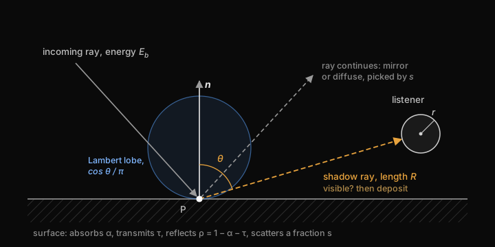
The share follows from two facts. A diffuse surface sends a fraction $\cos\theta/\pi$ of its reflected energy into each unit of solid angle, with $\theta$ measured from the surface normal. And a listener modelled as a sphere of radius $r$ at distance $R$ covers a solid angle of about $\pi r^2/R^2$. Multiply the two, and rain only the diffuse part $s$ of the reflection:
$$\Delta E_b = E_b\,\rho_b\,s\;\frac{\cos\theta}{\pi}\cdot\frac{\pi r^2}{R^2}\;e^{-m_b R} \;=\; E_b\,\rho_b\,s\,\cos\theta\,\frac{r^2}{R^2}\,e^{-m_b R}$$
The deposit is an estimate, not a transfer. The ray keeps its full reflected energy and carries on bouncing, and since nothing ever counts the ray itself arriving at the listener, nothing is counted twice.
Where the inverse-square law lives. It's tempting to also divide every deposit by $R^2$ to account for distance. Don't: the solid-angle term $r^2/R^2$ already is the inverse-square law. Applying it again counts distance twice.
Three practical details:
- The radius cancels. Divide the finished echogram by the number of rays and by $\pi r^2$ and you get energy per unit area, which doesn't depend on the $r$ you picked.
- Clamp $R$. Next to a wall, $R$ goes to zero and $r^2/R^2$ explodes. I clamp it at 0.5 m.
- Leave out the direct sound. The dry voice already delivers it; the reverb should only add what comes after.
One probe on its own is noisy, so probes are blended into a running average. The first probes are weighted equally and after that older probes fade out exponentially, so the estimate settles quickly and still follows you into the next room. Average the echogram, not the reverberation time computed from it: smoothing a number that was fitted to noisy data is worse than smoothing the data and fitting once.
One limitation to know about: only the diffuse part is rained. A path that reflects like a mirror all the way from the listener back to the listener never reaches the echogram until it scatters somewhere. That mostly affects the first few tens of milliseconds, so the start of the echogram is its least trustworthy part. Hybrid solvers handle early mirror reflections separately with image sources.
Reverberation time In progress
Schroeder integration
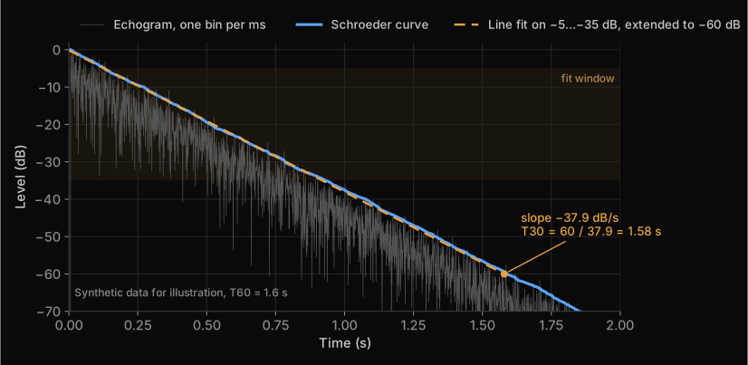
An echogram is far too spiky to read a decay from. Schroeder's method (1965) integrates it backwards: the energy decay curve at time $t$ is all the energy that still arrives after $t$.
$$\begin{aligned} \mathrm{EDC}(t) &= \int_t^{\infty} E(t')\,dt' \\ \mathrm{EDC}[k] &= \sum_{j \ge k} E[j] \\ L(t) &= 10\log_{10}\frac{\mathrm{EDC}(t)}{\mathrm{EDC}(0)} \end{aligned}$$
In decibels this is a smooth curve that starts at 0 dB and only goes down. For a single exponential decay it's a straight line.
EDT, T20 and T30
The reverberation time $T_{60}$ is how long a sound takes to decay by 60 dB. Hardly any measurement has 60 dB of clean decay, so ISO 3382-1 fits a straight line over part of the Schroeder curve and extrapolates:
| Measure | Fit range | What it describes |
|---|---|---|
| EDT | 0 to −10 dB | The start of the decay, which is closest to how reverberant a room sounds |
| T20 | −5 to −25 dB | The main decay |
| T30 | −5 to −35 dB | The main decay, over more range; needs the cleanest tail |
$$T = \frac{-60\ \text{dB}}{\text{slope in dB/s}}$$
The three are also a diagnostic. For a single-slope decay they agree. If T30 comes out shorter than T20, the tail is being cut off: the history is too short, too few rays survive, or a depth cap is in the way. The honest response is to report the value as invalid rather than return a wrong number, so my decay code checks that the curve actually reaches −35 dB inside the window and refuses to report T30 when it doesn't.
A cross-check from the rays: Eyring
The tracer also yields an analytical estimate almost for free. If rays hit a surface on average every $\bar\ell$ metres (the mean free path) and lose a fraction $\bar\alpha_b$ of their energy per hit, then after time $t$ they have made $ct/\bar\ell$ bounces:
$$E_b(t) = E_0\,(1-\bar\alpha_b)^{ct/\bar\ell}\,e^{-m_b c t}$$
Setting $E_b(T_{60}) = 10^{-6}E_0$ and solving for $T_{60}$ gives Eyring's formula:
$$T_{60} = \frac{6\ln 10}{c}\cdot\frac{\bar\ell}{-\ln(1-\bar\alpha_b) + m_b\bar\ell} \;\approx\; 0.161\,\frac{\bar\ell/4}{-\ln(1-\bar\alpha_b) + m_b\bar\ell}$$
For a room with volume $V$ and surface area $S$ the mean free path is $\bar\ell = 4V/S$, which turns this into the textbook form
$$T_{60} = \frac{0.161\,V}{-S\ln(1-\bar\alpha_b) + 4m_b V}$$
and for small $\bar\alpha_b$, where $-\ln(1-\bar\alpha_b) \approx \bar\alpha_b$, into Sabine's formula. The nice part: the probe measures $\bar\ell$ and a hit-weighted $\bar\alpha_b$ directly from its rays, so it gets an Eyring estimate without ever knowing $V$ or $S$, which you don't have for arbitrary level geometry.
Eyring assumes a diffuse field, with energy spread evenly and travelling in all directions. Real rooms, and certainly game levels full of corridors and connected spaces, often aren't like that. So the traced decay is the answer and Eyring is the sanity check. If the two disagree in a simple room, something is broken; if they disagree in a complicated one, that may be the whole point of tracing.
Next step: validating the whole chain in a shoebox room, where the answer is known. The traced mean free path should match $4V/S$ and the traced T30 should land close to Eyring. Until that passes, I treat every reverberation time the plugin reports as a measurement of the simulation, not of the room.
Making it audible: a feedback delay network In progress
There are two ways to turn all this into sound. Convolution plays the signal through an impulse response synthesized from the echogram. It's the most faithful, but the impulse response changes several times a second as you move, and crossfading between impulse responses without artifacts is a project in itself. A feedback delay network (FDN) is a parametric reverb: you give it a decay time per band and it produces a tail that matches, cheaply and smoothly. I'm starting with the FDN because it's easier to verify. Convolution stays an option once the physics is validated.
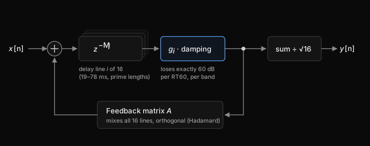
An FDN is a set of $N$ delay lines whose outputs are mixed and fed back into their inputs. With $v_i[n]$ the output of line $i$ and $M_i$ its length in samples:
$$v_i[n + M_i] = x[n] + \sum_{j=1}^{N} A_{ij}\,g_j\,v_j[n], \qquad y[n] = \frac{1}{\sqrt{N}}\sum_{i=1}^{N} g_i\,v_i[n]$$
With every $g_i = 1$ and an orthogonal matrix $A$, one that preserves energy, the network rings forever: it's lossless. The decay then comes entirely from the gains. After $T_{60}$ seconds the signal has to be 60 dB down, a factor $10^{-3}$ in amplitude, and a signal passes through line $i$ exactly $f_s T_{60}/M_i$ times in that time. So:
$$g_i = 10^{-3 M_i/(f_s T_{60})}$$
Because each gain is tied to its own line's length, every line decays along the same envelope, whatever its length. Frequency-dependent decay works the same way: the gain becomes a filter whose magnitude at frequency $f$ is $10^{-3M_i/(f_s T_{60}(f))}$. I approximate that with a one-pole lowpass per line, with the gain set from the mid-band decay time and the damping from the tilt between the low and high bands. Jot and Chaigne (1991) describe this design in detail.
The rest of the design is about density. The feedback matrix is a normalized Hadamard matrix, built by doubling:
$$H_1 = \begin{pmatrix} 1 \end{pmatrix}, \qquad H_{2N} = \frac{1}{\sqrt{2}}\begin{pmatrix} H_N & H_N \\ H_N & -H_N \end{pmatrix}$$
It mixes every line into every other line with equal strength, and it can be applied as a fast transform in $N\log_2 N$ additions instead of a full matrix multiply. The 16 delay lengths are different prime numbers of samples between 19 and 78 ms, so their echoes never line up into an audible pattern. The predelay, the gap before the reverb starts, comes from the first bin of the echogram that holds energy.
Where it stands: the reverb is audible and its decay follows the tracer, but it isn't finished. The output is still mono, the same signal on both channels, which collapses the tail into the middle of your head; the plan is to send half of the lines to each ear. Changing the predelay while the reverb plays may be what causes occasional clicks, so predelay changes will get a crossfade. The FDN also has a self-test: it feeds itself an impulse with a hand-typed $T_{60}$, runs the same Schroeder analysis on its own output and checks that it measures what it was asked for. That way a bug in the tracer can't be hidden by tuning the reverb, or the other way around.
Keeping the audio thread fed
Audio has a hard deadline. The audio callback has to deliver a buffer every few milliseconds, and if it waits on anything, you hear a dropout rather than a hitch. Ray tracing takes far longer than a buffer, so the two never share a lock.
- Tracing runs on background tasks: per-source occlusion about 30 times a second, the room probe 4 times a second.
- Each task publishes only small derived results, like six band values or a few decay times, through a seqlock. The writer bumps a version counter before and after writing; a reader copies the data and simply retries if the counter was odd or changed while it was copying. The audio thread never waits for the tracer.
- Nothing jumps on the audio side. Gains and filter coefficients ramp across a buffer, and reverb settings are only updated when they change by more than a small threshold.
Where it stands
| Part | Technique | Status |
|---|---|---|
| Acoustic materials | Measured absorption tables, energy budget per band | Working |
| Transmission | Sharp's model, single and double leaf | Working |
| Occlusion | Direct path plus next-event estimation, three-band voice filter | Working |
| Distance and air | Inverse-square law, ISO 9613-1 air absorption (the direct path still uses a simpler lowpass) | Working |
| Echogram | Diffuse rain, Russian roulette, running average | Working |
| Reverberation time | Schroeder integration, EDT, T20, T30, Eyring cross-check; not validated yet | In progress |
| Reverb | 16-line FDN with per-band decay; audible, mono, being tuned | In progress |
| Validation | Shoebox room: traced mean free path against 4V/S, T30 against Eyring | Planned |
| Stereo reverb | Decorrelated left and right outputs | Planned |
| Diffraction | Sound bending around edges and through openings | Planned |
| Spatialization | Direction of arrival for reflections, HRTFs | Planned |
| Multiple rooms | A late field per room instead of one per listener | Planned |
| Performance | Profiling instead of estimates | Planned |
Known limitations
- Low frequencies. Rays can't represent diffraction or room modes, and below a few hundred hertz both matter.
- One late field per listener. The probe describes the room you're standing in. A source in the next room excites a different reverb, which a single shared field can't express.
- Transmission inputs. Sharp's model gets asked about porous materials, small objects and gaps it wasn't built for, with thicknesses that are often invented.
- Scattering per material instead of per surface shape.
- Occlusion is a heuristic: a plausible estimate per band, not a solution of energy transport.
References
- B. H. Sharp (1978), "Prediction Methods for the Sound Transmission of Building Elements", Noise Control Engineering 11(2), 53–63
- M. Long, Architectural Acoustics, chapter 9, "Sound Transmission Loss" (Elsevier)
- INSUL, technical background on single and double panel transmission loss
- H. Kuttruff, Room Acoustics (CRC Press)
- M. Vorländer, Auralization (Springer)
- M. R. Schroeder (1965), "New Method of Measuring Reverberation Time", Journal of the Acoustical Society of America 37, 409–412
- C. F. Eyring (1930), "Reverberation Time in 'Dead' Rooms", Journal of the Acoustical Society of America 1, 217–241
- J.-M. Jot and A. Chaigne (1991), "Digital Delay Networks for Designing Artificial Reverberators", 90th AES Convention
- D. Schröder (2011), Physically Based Real-Time Auralization of Interactive Virtual Environments, PhD thesis, RWTH Aachen (diffuse rain)
- E. Veach (1997), "Robust Monte Carlo Methods for Light Transport Simulation", PhD thesis, Stanford (next-event estimation, Russian roulette)
- ISO 354 (absorption in a reverberation room), ISO 17497-1 (scattering), ISO 9613-1 (air absorption), ISO 3382-1 (room acoustic parameters)
- Steam Audio, an open-source reference for how a production system handles the same problems